NSPLINE
=NSPLINE(known_xs, known_ys, [x])
| Argument | Description | Example |
|---|---|---|
| known_xs | The x-values of the control points in increasing order | {2;4;8;10} |
| known_ys | The y-values of the control points | {3;1;5;5} |
| x | [optional] Values of x to interpolate | {2;2.1;...;9.9;10} |
In the template file, navigate to the Polynomials worksheet to see the NSPLINE function in action.
Description
NSPLINE is used for natural cubic spline interpolation. Like CSPLINE, it creates a cubic piecewise polynomial that passes through a given set of control points. Both the first and second derivatives are continuous and the second derivative at the end points is zero.
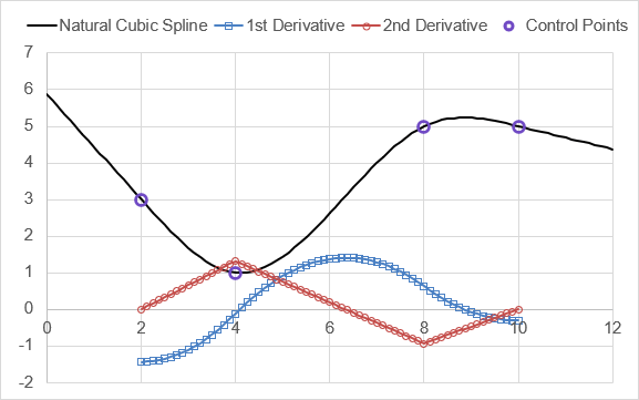
The image below shows an example of a natural cubic spline through 4 control points, along with the first and second derivatives, which you can observe are indeed continuous.

Note that PPVAL does not extrapolate. This is why the derivatives of the spline in the above image are evaluated only between the control points.
The default output of NSPLINE is a piecewise polynomial data structure array that can be used by PPVAL for interpolation.
=LET(
    known_xs, {2;4;8;10},
    known_ys, {3;1;5;5},
    NSPLINE(known_xs,known_ys)
)

Result: pp_array
{2,  0.109375,        0, -1.4375,  3;
 4,  -0.09375,  0.65625,  -0.125,  1;
 8,  0.078125, -0.46875,   0.625,  5;
10,        "",       "",      "", ""}
If the x parameter is not blank, then the output will be a vector of interpolated values corresponding to the values in x. The following example interpolates the natural spline at 49 values of x between 0 and 12 (NSPLINE can extrapolate).
=LET(
    known_xs, {2;4;8;10},
    known_ys, {3;1;5;5},
    interp_x, LINSPACE(0,12,49),
    NSPLINE(known_xs,known_ys,interp_x)
)

Result: {5.875; 5.5156; ... ; 4.453; 4.375}
Why is it Called Natural?
A flexible ruler (with constant thickness and material properties) that passes through the control points without being clamped (meaning that the slope is not constrained by an outside force) will follow the shape of the natural spline because this shape minimizes bending energy. Thus, it is the "natural" state of the flexible ruler. Note that the control points only constrain the vertical position, so the ruler would be allowed to slip and rotate at each point as needed.
The youtube series Splines in 5 Minutes by professor Steve Seitz does a very good job of explaining this concept, and even shows an actual experiment with duck weights and a flexible ruler.
The constraint that the second derivative is zero at the end points means that the curvature is zero (no bending) at the end points. As a result, the ruler would extend unbent beyond the first and last control point, so NSPLINE extrapolates based on a straight line if values of x are <x1 or >xn. The slope at the end points is not specified, but can be determined by finding the derivative of the spline at the ends using PPDER.
How it Works
The NSPLINE function uses the algorithm from the wikipedia article in reference [1]. See the more general SPLINE function for an algorithm that solves a system of constraint equations.
Lambda Formula
This code for using NSPLINE in Excel is provided under the License as part of the LAMBDA Library, but to use just this function, you may copy the following code directly into your spreadsheet.
Code for AFE Workbook Module (Excel Labs Add-in)
/**
 * Natural Cubic Spline - Creates a C2 Interpolating Spline with d2y/dx2=0 at the endpoints.
 */
/*
 * Inputs:
 *   known_xs: A column vector of known x-values (independent variable).
 *   known_ys: A column vector of known y-values (dependent variable).
 *   [x]: Optional. The value(s) to interpolate. If omitted, returns the piecewise polynomial parameters.
 *
 * Outputs:
 *   Returns the interpolated value(s) for x, or the piecewise polynomial coefficients if x is omitted.
 *
 * Notes:
 *   - Ensures C2 continuity and natural spline conditions (second derivative is zero at endpoints).
 *   - Supports multiple x values for interpolation.
 *   - Returns 0 for extrapolated values beyond the range of known_xs and known_ys.
 *
 * Requires: POLYVAL, POLYDER, PPVAL
 */
NSPLINE = LAMBDA(known_xs, known_ys, [x],
LET(
    doc, "https://www.vertex42.com/lambda/nspline.html",

    // Step 1: Ensure xs and ys are column vectors
    xs, IF(AND(ROWS(known_xs) = 1, COLUMNS(known_xs) > 1), TRANSPOSE(known_xs), known_xs),
    ys, IF(AND(ROWS(known_ys) = 1, COLUMNS(known_ys) > 1), TRANSPOSE(known_ys), known_ys),

    // Step 2: Calculate differences between consecutive x-values (h) and other preliminaries
    h, DROP(xs, 1) - DROP(xs, -1),
    n, ROWS(xs),
    alpha, 3 / DROP(h, 1) * (DROP(ys, 2) - DROP(DROP(ys, 1), -1))
        - 3 / DROP(h, -1) * (DROP(DROP(ys, 1), -1) - DROP(ys, -2)),

    // Step 3: Solve the tridiagonal system for the spline coefficients
    l_mu_z, REDUCE({1, 0, 0}, SEQUENCE(n - 2, 1, 2, 1), LAMBDA(acc, i,
        LET(
            mu_o, INDEX(acc, i - 1, 2),
            z_o, INDEX(acc, i - 1, 3),
            li, 2 * (INDEX(xs, i + 1) - INDEX(xs, i - 1)) - INDEX(h, i - 1) * mu_o,
            mui, INDEX(h, i) / li,
            zi, (INDEX(alpha, i - 1) - INDEX(h, i - 1) * z_o) / li,
            ret, VSTACK(acc, HSTACK(li, mui, zi)),
            IF(i = n - 1, VSTACK(ret, {1, 0, 0}), ret)
        )
    )),
    li, INDEX(l_mu_z, , 1),
    mui, INDEX(l_mu_z, , 2),
    zi, INDEX(l_mu_z, , 3),

    // Step 4: Back-substitute to compute the cubic coefficients
    d_c_b, REDUCE({0, 0, 0}, SEQUENCE(n - 1, 1, n - 1, -1), LAMBDA(acc, j,
        LET(
            co, INDEX(acc, 1, 2),
            cj, INDEX(zi, j) - INDEX(mui, j) * co,
            bj, (INDEX(ys, j + 1) - INDEX(ys, j)) / INDEX(h, j) - 1 / 3 * INDEX(h, j) * (co + 2 * cj),
            dj, (co - cj) / (3 * INDEX(h, j)),
            ret, VSTACK(HSTACK(dj, cj, bj), acc),
            ret
        )
    )),
    pp, MAP(HSTACK(xs, DROP(HSTACK(d_c_b, ys), -1)), LAMBDA(cell, IFERROR(cell, ""))),

    // Step 5: Handle extrapolation (linear interpolation at the endpoints)
    m_1, POLYVAL(POLYDER(DROP(CHOOSEROWS(pp, 1), 0, 1)), 0),
    b_1, INDEX(known_ys, 1, 1) - m_1 * INDEX(known_xs, 1, 1),
    m_n, POLYVAL(POLYDER(DROP(CHOOSEROWS(pp, n - 1), 0, 1)), INDEX(pp, n, 1) - INDEX(pp, n - 1, 1)),
    b_n, INDEX(known_ys, n, 1) - m_n * INDEX(known_xs, n, 1),

    // Step 6: Interpolate or return coefficients
    IF(ISOMITTED(x), pp,
        (x < INDEX(known_xs, 1, 1)) * (m_1 * x + b_1) +
        (x > INDEX(known_xs, n, 1)) * (m_n * x + b_n) +
        IFERROR(PPVAL(pp, x), 0)
    )
));
NSPLINE Examples
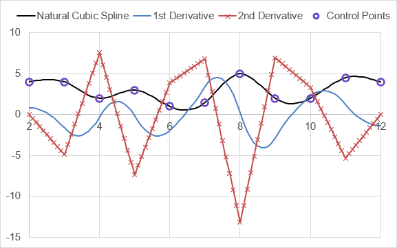
This is the example from the PPDER documentation.
=LET(
    x_cpts, {2;3;4;5;6;7;8;9;10;11;12},
    y_cpts, {4;4;2;3;1;1.5;5;2;2;4.5;4},
    pp_spline, NSPLINE(x_cpts,y_cpts),
    x_interp, LINSPACE(2,12,101),
    y_interp, PPVAL(pp_spline,x_interp),
    dy_interp, PPVAL( PPDER(pp_spline),x_interp),
    d2y_interp, PPVAL( PPDER(PPDER(pp_spline)),x_interp),
    HSTACK(x_interp,y_interp,dy_interp,d2y_interp)
)

Result: (see graph below)

See Also
PPVAL, POLYDER, POLYVAL, CSPLINE, SPLINE, PPDER, PPINT
- [1] Wikipedia - Spline
- Wikipedia - Spline Interpolation
- Natural Spline Interpolation (PDF), Eberly, D., 2008.
