FDIFF - Finite Difference
=FDIFF(ys, [h], [n])
| Argument | Description | Example |
|---|---|---|
| ys | A column vector of known y values | {2;5;11;20;30} |
| h | (default=1) The step size of x, Δx | 1 |
| n | (default=1) The n-th Derivative (1, 2, 3 or 4) | 1 |
In the template file, navigate to the Calc worksheet to see the FDIFF function in action.
Description
FDIFF uses 2nd-order Finite Differences to estimate the nth-derivative \(d^ny/dx^n\) of a set of y values with a constant step size, \(h={\Delta}x\). The derivatives are evaluated at each of the points corresponding to yi. The result is a vector the same length as ys.
The function is defined for the 1st through the 4th derivatives, and is only valid for evenly spaced points (constant Δx). It assumes that the y-values are already ordered based on x increasing with step size h. The x values do not need to be provided, because the function depends only on h (not the values of x). If h is blank, it is assumed to be Δx=1.
The function uses a Forward Difference Derivative (FDD) for the first point(s), a Central Difference Derivative (CDD) for the middle points, and a Backward Difference Derivative (BDD) for the last point(s). For quadratic-level accuracy, the function uses n+2 points. The set of points is referred to as the "stencil" and the values of y within the stencil are multiplied by a set of coefficients shown below.
The coefficients used in FDIFF were obtained using the Finite Difference Coefficients Calculator by Cameron Taylor. The following are the formulas used in this function (where m is the number of values in ys):
Forward Difference Derivative
$$ y'_1 = \left(-3y_1+4y_2-1y_3\right)/(2h)$$ $$ y''_1 = \left(2y_1-5y_2+4y_3-1y_4\right)/(h^2)$$ $$ y'''_1 = \left(-5y_1+18y_2-24y_3+14y_4-3y_5\right)/ (2h^3)$$ $$ y'''_2 = \left(-3y_1+10y_2-12y_3+6y_4-1y_5\right)/ (2h^3)$$ $$ y''''_1 = \left(3y_1-14y_2+26y_3-24y_4+11y_5-2y_6\right)/ (h^4)$$ $$ y''''_2 = \left(2y_1-9y_2+16y_3-14y_4+6y_5-1y_6\right)/ (h^4)$$Central Difference Derivative
$$ y'_i = \left(-1y_{i-1}+0y_i+1y_{i+1}\right)/(2h)$$ $$ y''_i = \left(1y_{i-1}-2y_i+1y_{i+1}\right)/(h^2)$$ $$ y'''_i = \left(-1y_{i-2}+2y_{i-1}+0y_i-2y_{i+1}+1y_{i+2})\right)/ (2h^3)$$ $$ y''''_i = \left(1y_{i-2}-4y_{i-1}+6y_i-4y_{i+1}+1y_{i+2}\right)/ (h^4)$$Backward Difference Derivative
$$ y'_m = \left(1y_{m-2}-4y_{m-1}+3y_m\right)/(2h)$$ $$ y''_m = \left(-1y_{m-3}+4y_{m-2}-5y_{m-1}+2y_m\right)/h^2$$ $$ y'''_{m-1} = \left(1y_{m-4}-6y_{m-3}+12y_{m-2}-10y_{m-1}+3y_m\right)/ (2h^3)$$ $$ y'''_m = \left(3y_{m-4}-14y_{m-3}+24y_{m-2}-18y_{m-1}+5y_m\right)/ (2h^3)$$ $$ y''''_{m-1} = \left(-1y_{m-5}+6y_{m-4}-14y_{m-3}+16y_{m-2}-9y_{m-1}+2y_m\right)/ (h^4)$$ $$ y''''_m = \left(-2y_{m-5}+11y_{m-4}-24y_{m-3}+26y_{m-2}-14y_{m-1}+3y_m\right)/ (h^4)$$Higher-Order Derivatives: If you need higher than a 4th derivative, you can use PDIFF for a more general solution. The calculator by Cameron Taylor can also generate coefficients for higher orders if you need them.
Comparison to PDIFF
The results of FDIFF(ys,h,n) are the same as PDIFF(xs,ys,,n) when the points are spaced evenly (Δx=h), and the algorithm should be quite a bit faster. My tests with TIMER showed FDIFF running about 2-5 times faster. A more rigorous analysis of the computational effort would be useful.
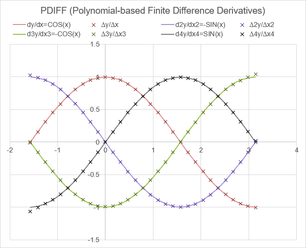
The example below shows the results of PDIFF for y=SIN(x) which has derivatives y'=COS(x), y''=-SIN(x), y'''=-COS(x), y''''=SIN(x). See the example below for how these results are generated with FDIFF.

We've used "x" shaped markers for all of these points because when comparing data points with a high degree of precision, using different shapes and sizes of markers in Excel can inaccurately represent true positions. For example, the exact center of a square marker may shift depending on the size of the marker. Excel charts are not known for their scientific precision, but we are also dealing with a limit of pixel-level precision.
1st-Order FDD and BDD
The following formulas are commonly used for the Forward Difference Derivative (FDD) and the Backward Difference Derivative (BDD), but note that these use only 2 points and are only linear approximations rather than the quadratic versions above.
$$FDD=\frac{y_2-y_1}{x_2-x_1}, BDD=\frac{y_m-y_{m-1}}{x_m-x_{m-1}} $$Note: A quadratic approximation does not guarantee a better estimate of the derivative at the edges, because it depends on the true shape of the curve at those points.
Lambda Formula
This code for using FDIFF in Excel is provided under the License as part of the LAMBDA Library, but to use just this function, you may copy the following code directly into your spreadsheet.
Code for AFE Workbook Module (Excel Labs Add-in)
/**
* Calculate the n-th Finite Difference Derivative assuming uniform spacing h
*/
FDIFF = LAMBDA(ys,[h],[n],
LET(doc,"https://www.vertex42.com/lambda/fdiff.html",
    n,IF(ISBLANK(n),1,n),
    h,IF(ISBLANK(h),1,h),
    m,ROWS(ys),
    MAKEARRAY(m,1,LAMBDA(i,j,
        SWITCH(n,
            1,SWITCH(i,
                1,SUMPRODUCT({-3;4;-1},INDEX(ys,1):INDEX(ys,3))/(2*h),
                m,SUMPRODUCT({1;-4;3},INDEX(ys,m-2):INDEX(ys,m))/(2*h),
                SUMPRODUCT({-1;0;1},INDEX(ys,i-1):INDEX(ys,i+1))/(2*h)
            ),
            2,SWITCH(i,
                1,SUMPRODUCT({2;-5;4;-1},INDEX(ys,1):INDEX(ys,4))/(h^2),
                m,SUMPRODUCT({-1;4;-5;2},INDEX(ys,m-3):INDEX(ys,m))/(h^2),
                SUMPRODUCT({1;-2;1},INDEX(ys,i-1):INDEX(ys,i+1))/(h^2)
            ),
            3,SWITCH(i,
                1,SUMPRODUCT({-5;18;-24;14;-3},INDEX(ys,1):INDEX(ys,5))/(2*h^3),
                2,SUMPRODUCT({-3;10;-12;6;-1},INDEX(ys,1):INDEX(ys,5))/(2*h^3),
                m-1,SUMPRODUCT({1;-6;12;-10;3},INDEX(ys,m-4):INDEX(ys,m))/(2*h^3),
                m,SUMPRODUCT({3;-14;24;-18;5},INDEX(ys,m-4):INDEX(ys,m))/(2*h^3),
                SUMPRODUCT({-1;2;0;-2;1},INDEX(ys,i-2):INDEX(ys,i+2))/(2*h^3)
            ),
            4,SWITCH(i,
                1,SUMPRODUCT({3;-14;26;-24;11;-2},INDEX(ys,1):INDEX(ys,6))/(h^4),
                2,SUMPRODUCT({2;-9;16;-14;6;-1},INDEX(ys,1):INDEX(ys,6))/(h^4),
                m-1,SUMPRODUCT({-1;6;-14;16;-9;2},INDEX(ys,m-5):INDEX(ys,m))/(h^4),
                m,SUMPRODUCT({-2;11;-24;26;-14;3},INDEX(ys,m-5):INDEX(ys,m))/(h^4),
                SUMPRODUCT({1;-4;6;-4;1},INDEX(ys,i-2):INDEX(ys,i+2))/(h^4)
            ),
            "Error: Invalid Integer n, 1<=n<=4"
        )
    ))
));
Named Function for Google Sheets
Name: FDIFF
Description: Calculates n-th Finite Difference Derivatives assuming uniform spacing
Arguments: start, end, n (see above for descriptions and example values)
Function:
[same as the Excel version]
FDIFF Examples
Test: Copy and Paste this LET function into a cell
=LET(
    x, LINSPACE(-PI()/2,PI(),31),
    y, SIN(x),
    h, INDEX(x,2)-INDEX(x,1),
    VSTACK(
    HSTACK("COS(x)","∆y/∆x","-SIN(x)","∆2y/∆x2","-COS(x)","∆3y/∆x3","SIN(x)","∆4y/∆x4"),
    HSTACK(
      COS(x),FDIFF(y,h,1),
      -SIN(x),FDIFF(y,h,2),
      -COS(x),FDIFF(y,h,3),
      SIN(x),FDIFF(y,h,4)
    )
    )
)
Test: Copy and Paste this LET function into a cell
=LET(
    x, LINSPACE(-PI()/2,PI(),31),
    y, SIN(x),
    h, INDEX(x,2)-INDEX(x,1),
    VSTACK(
    HSTACK("COS(x)","∆y/∆x","-SIN(x)","∆2y/∆x2","-COS(x)","∆3y/∆x3","SIN(x)","∆4y/∆x4"),
    HSTACK(
      COS(x),FDIFF(y,h,1),
      -SIN(x),FDIFF(FDIFF(y,h,1),h,1),
      -COS(x),FDIFF(FDIFF(FDIFF(y,h,1),h,1),h,1),
      SIN(x),FDIFF(FDIFF(FDIFF(FDIFF(y,h,1),h,1),h,1),h,1)
    )
    )
)
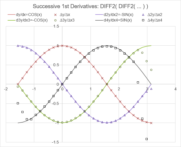
The answer is "they are not the same," as shown in the following chart. Note that especially on the edges, the errors compound rather quickly.

Compare \(y''_i\) to the following formula for \(f'(f'(x_i))\) derived from successive use of \(y'_i\).
$$ y'_i = \left(-1y_{i-1}+0y_i+1y_{i+1}\right)/(2h)$$ $$ y''_i = \left(1y_{i-1}-2y_i+1y_{i+1}\right)/(h^2)$$ $$f'(f'(x_i)) = \left(-1y_{i-2}+0y_{i-1}-2y_i+0y_{i+1}+1y_{i+2}\right)/(4h^2)$$Notice that successive use of \(y'_i\) expands the stencil more rapidly, which in theory should produce less accurate results. To achieve more accurate estimates of derivatives, we would want higher order fits using smaller values of h, though if h is too small we run into numerical percision error. A rough rule of thumb for the size of h in Excel is \(h \approx x\sqrt{10^{-16}}\).
=LET(
    h_vec, LOGSPACE(-1,-15,15),
    x, 1,
    fx, SIN(x),
    fpx, COS(x),
    fxmh_vec, SIN(x-h_vec),
    fxph_vec, SIN(x+h_vec),
    dydx_vec,MAKEARRAY(ROWS(h_vec),1,LAMBDA(i,j,
        LET(ys,VSTACK( INDEX(fxmh_vec,i),fx,INDEX(fxph_vec,i) ),
            h,INDEX(h_vec,i),
            INDEX( FDIFF(ys,h,1), 2)
        )
    )),
    error_vec,ABS(dydx_vec-fpx),
    VSTACK(
        HSTACK("h","error"),
        HSTACK(h_vec,error_vec)
    )
)

Result:
{ "h",   "error";
1E-01, 9.001E-04;
1E-02, 9.005E-06;
1E-03, 9.005E-08;
1E-04, 9.004E-10;
1E-05, 1.114E-11;
1E-06, 2.772E-11;
1E-07, 1.943E-10;
1E-08, 2.581E-09;
1E-09, 2.970E-09;
1E-10, 5.848E-08;
1E-11, 1.169E-06;
1E-12, 1.227E-05;
1E-13, 1.788E-04;
1E-14, 3.707E-04;
1E-15, 1.481E-02}
In this particular example, it looks like the the optimal value for h is around 0.00001 or 0.000001.
See Also
DIFF, FDIFF, PDIFF, TRAPZ, SIMPSON
