BOOKMARK - Create a Dynamic HYPERLINK
=BOOKMARK(cell)
| Argument | Description | Example |
|---|---|---|
| cell | The cell you want to link to | Sheet1!B50 |
In the template file, navigate to the General worksheet to see the BOOKMARK function in action.
Description
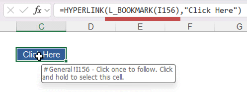
The BOOKMARK function helps you create the string used for the link_location in the HYPERLINK function to make a clickable link to another cell in your workbook. This is the function used within the lambda library download file to navigate to the different example functions. The usage is very simple and only requires you to reference "go to" cell one time:
=HYPERLINK( BOOKMARK(cell_ref), "click here" )

You may be wondering why you'd want to use a lambda function for this, rather than one of the other methods. So, let's talk about the 3 methods for inserting a bookmark in Excel:
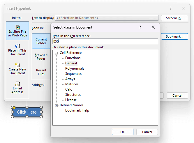
Method 1: Insert Hyperlink > Bookmark
You can add custom navigation elements, including custom shapes that act as buttons, to your Excel workbook using the Insert Hyperlink (Ctrl+k) command.
The problem: The bookmark is a fixed location such as Sheet1!A50, so if you insert new rows above A50 in Sheet1, your bookmark will not move with your data (the hyperlink remains pointing to cell A50).

Method 2: Insert Hyperlink > Bookmark > Defined Name
This works. To create a dynamic bookmark that moves with your data, you can use the Name Manager to create a named range such as "bookmark_help" that links to Sheet1!A50. Then, you can select that Defined Name using Ctrl+k (see the image above).
The problem: You can end up having a lot of named ranges in your workbook, which can get especially messy if you start copying worksheets. This is a great method if you don't mind using named ranges. It also still works with shape objects as buttons.
Method 3: Use the HYPERLINK function
You can use the HYPERLINK function within a cell to create a clickable link or "bookmark" to a another cell in your workbook. This requires using a very specific syntax for the link_location in the HYPERLINK function, including the beginning "#" and the "!" between the sheet name and cell address. Also, remember to use the single quotes for sheet names that include spaces:
=HYPERLINK("#'Sheet Name'!B10","click here")
If you "hard code" the Sheet Name and the cell address B10 into your HYPERLINK function, then your link is still not dynamic. The reference will not move with your data. So, to create a dynamic link to a particular cell, you'll need a way to (1) get the worksheet name in case the worksheet name changes and (2) get the cell address B10. The BOOKMARK function does this for you.
How it Works
To get the cell address by referencing a cell, use the ADDRESS function. ADDRESS can return a text version of the cell address as A50, $A$50 or even R[50]C[1]. If we want to get the address string for a particular cell_ref, we use:
=ADDRESS(ROW(cell_ref),COLUMN(cell_ref),4)
Result: If cell_ref is Sheet!A50, the result will be A50
The ADDRESS function also includes an optional [sheet_text] parameter which allows you to specify the worksheet name as a string.
To get the worksheet name by referencing a cell, use the CELL function. CELL("filename",cell_ref) will return a string that looks like this: "[c:/longpath/]Sheet Name". We can use TEXTAFTER to get the sheet name:
=TEXTAFTER(CELL("filename",cell_ref),"]")
Result: If cell_ref is 'Sheet One'!A50, the result will be "Sheet One"

NOTE: CELL("filename",cell_ref) returns "" if the file is not saved yet.
Note: The [sheet_text] parameter in the ADDRESS function automatically adds the single quotes around a sheet name string if it contains spaces.
The final formula, using LET to avoid referencing the cell 3 separate times, isn't too terrible. I've used "c" instead of "cell_ref" to make the formula more concise.
=LET(c,A50,"#"&ADDRESS(ROW(c),COLUMN(c),4,1,TEXTAFTER(CELL("filename",c),"]")))
Lambda Formula
This code for using BOOKMARK in Excel is provided under the License as part of the LAMBDA Library, but to use just this function, you may copy the following code directly into your spreadsheet.
Code for AFE Workbook Module (Excel Labs Add-in)
/**
* Create a hyperlink to a specific cell in the workbook
*/
BOOKMARK = LAMBDA(cell,
LET(doc,"https://www.vertex42.com/lambda/bookmark.html",
    "#"&ADDRESS(ROW(cell),COLUMN(cell),4,1,TEXTAFTER(CELL("filename",cell),"]"))
));
Named Function for Google Sheets
The HYPERLINK function in Google Sheets works a bit differently because to hyperlink to a different worksheet requires you to use the gid of the worksheet, not the worksheet name. The gid for the worksheet is found in the URL for that worksheet. As far as I know, there isn't a formula or function that can automatically get the gid.
=HYPERLINK( BOOKMARK(A1,"12345"),"click here")

BOOKMARK will return a string that looks like this: "#gid=12345&range=A1"
Name: BOOKMARK
Description: Creates the link_location for HYPERLINK to navigate to a cell in the workbook
Arguments: cell, gid
Function:

=LET(doc,"https://www.vertex42.com/lambda/bookmark.html",
"#gid="&gid&"&range="&ADDRESS(ROW(cell),COLUMN(cell),4)
)
