Creating Business Forms with Customizable Lists

Spreadsheets are great tools for creating business forms such as invoices, order forms, or expense reports. If you use a form like this routinely, you may come across times when it would be handy to select items from a drop-down list and have other information update automatically. Let me give an example ...

Today I added a new purchase order template to my website that includes a customizable price list. Instead of manually entering the description, item #'s, and prices, you can select an item from an Excel drop-down menu as shown in the image below:

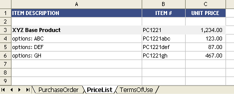
The list can be customized in a separate worksheet as shown in the following image:

In this case, the purpose isn't just to select items from a list. We want the Item # and the Unit Price to update automatically based on whatever item was selected.

How It's Done

I'm going to give a general outline for how this is done. There are basically 3 steps:

#1 - Create the List

This part's easy. Just add a worksheet and put some labels at the top of the columns and start adding data, just like in the PriceList worksheet shown above.

#2 - Add a Drop-Down List to Your Form

To create the drop-down list, we can use the Data Validation feature in Excel. For detailed instructions on this procedure, see my article Create a Drop-Down List using Data Validation. (You'll need to review that article to understand the rest of this post). The important thing to get out of that article is that you need to use a named range if your customizable list is on a separate worksheet.

You don't have to be fancy with your named range. In the price list example above, I could define the range as =PriceList!$A$1:$A$300, but then I'd end up showing 300 rows in my drop-down list instead of just the 6 I needed (the rest of the 294 rows would be blank). Or, I could define it as =PriceList!$A$1:$A$6. In that case, when I edited the price list, I'd need to make sure to either insert rows above A6 or change the definition of the named range after adding on to the end of the list. In a template, that can of editing is usually a bit much to ask of the user.

A more advanced technique, which also makes things easier for the user, is to use something we call a dynamic named range, or a range that adjusts its size automatically. In this case, we want the range to extend only to the last non-blank row from our price list. So, we use a formula like this for the named range: =OFFSET(PriceList!$A$1,0,0,MATCH(REPT("z",255),PriceList!$A:$A),1)

If you want to learn more about that technique, see the article Formulas for Dynamic Named Ranges.

#3 - Automatically Add the Item # and Unit Price

To populate the Item # and Unit Price columns based on what we select from the drop-down list, we can use the LOOKUP() or INDEX(MATCH()) techniques. I prefer the INDEX(MATCH()) approach. The formula for the Unit Price looks like something like this
=INDEX(PriceList!C:C,MATCH(B21,PriceList!A:A,0))

In English, this is effectively saying "Select the unit price from the PriceList worksheet where the corresponding description matches what we just selected from the drop-down list".

Other Examples

If you'd like to see examples in spreadsheets that you can download for free, you can take a look at the money management template and meal planners.