L_PDIFF
=L_PDIFF(xs, ys, [nth_deriv], [order])
| Argument | Description | Example |
|---|---|---|
| xs | A column vector of known x values | {1;2;3;4;5} |
| ys | A column vector of known y values | {2;5;11;20;30} |
| nth_deriv | (default=1) The derivative to approximate | 1 |
| order | (default=2) The order of accuracy | 2 |
Requires: L_POLYFIT, L_POLYDER, L_POLYVAL
Description
L_PDIFF is a polynomial-based finite difference function for estimating numeric derivatives given an ordered set of x and y=f(x) values. The spacing of the x values does not need to be uniform. Using the defaults, L_PDIFF(xs,ys) returns the approximation of the 1st derivative \(y'(x_i)\) at all values of xs.
For ease of implementation combined with the flexibility to choose the order of accuracy, PDIFF uses a polynomial fit of a stencil that consists of a number of closest ordered (x,y) points (making it unnecessary to use different formulas for edge points).
For the n-th derivative, the stencil is n+order points fit with an n+order-1 degree polynomial. For example, the 2nd derivative at 2nd-order accuracy requires 2+2=4 points and is fit with a 3rd-degree polynomial. Increasing the order of accuracy increases the number of stencil points and the degree of the polynomial. Increasing the order of accuracy does not necessarily guarantee increased accuracy, because the additional points are further away from x.
The example below shows the results of L_PDIFF for y=SIN(x) which has derivatives y'=COS(x), y''=-SIN(x), y'''=-COS(x), y''''=SIN(x). This example uses 2nd-order accuracy.
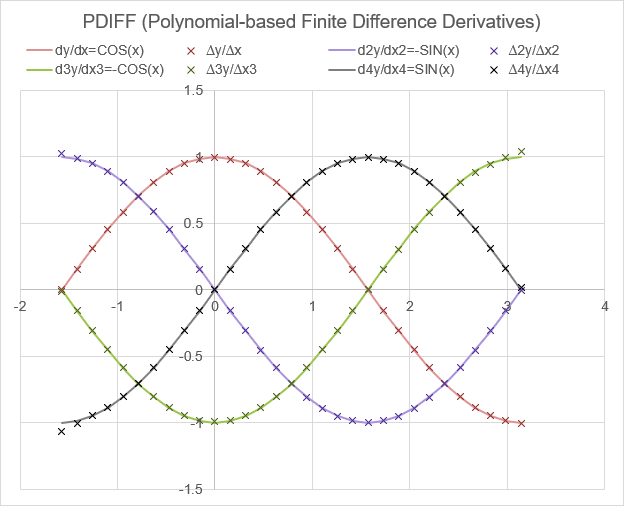
Note that the step size of x in this example is not very small (about 0.157). Using a smaller step size should increase accuracy, provided that the step size is not too small. If the step size is too small, you can run into machine precision errors. See FDIFF for an example of evaluating an optimal step size.
How it Works
This algorithm is actually only a small variation on the PINTERP algorithm used for piecewise polynomial interpolation. The main difference is the calculation of the derivatives of the interpolating polynomial using L_POLYDER.
To calculate the n-th finite difference derivative at the value x:
- Determine the stencil (points to include in the polynomial fit) by finding the n+order closest points to xi.
- Shift the stencil x-values to 0 via xs-xo where xo is the minimum x value in the stencil. This is done to avoid numerical instability that can occur at large |x| values.
- Use L_POLYFIT to fit an interpolating polynomial of degree n+order-1 to these n+order points.
- Use L_POLYDER recursively n times to calculate the n-th derivative of the interpolating polynomial.
- Use L_POLYVAL to estimate the derivative \( {\Delta}^ny/{\Delta}x^n \) at the value x-xo.
Comparison to FDIFF
If the xs values are evenly spaced (Δx = h), PDIFF(xs,ys,n,2) should produce the same results as FDIFF(ys,h,n).
Computational Efficiency
Although the function is generalized for nonuniform spacing and a specified order of accuracy, it is not the most computationally efficient. In fact, reference [2, pg 10] calls this approach cumbersome. However, it is easy to code with the use of the L_POLYFIT, L_POLYDER, and L_POLYVAL functions. See L_FDIFF for a more efficient algorithm that calculates up to the 4th derivative at 2nd-order accuracy (and is about 2-5 times faster).
Lambda Formula
This code for using L_PDIFF in Excel is provided under the License as part of the LAMBDA Library, but to use just this function, you may copy the following code directly into your spreadsheet.
Code for AFE Workbook Module (Excel Labs Add-in)
/**
* Calculate the nth-Derivative of y(x) using a polynomial-based Finite Difference approximation
* Default: Finds the 1st derivative at 2nd-order accuracy
*/
L_PDIFF = LAMBDA(xs,ys,[nth_deriv],[order],
LET(doc,"https://www.vertex42.com/lambda/pdiff.html",
    n,IF(ISBLANK(nth_deriv),1,nth_deriv),
    order,IF(ISBLANK(order),2,order),
    BYROW(xs,LAMBDA(x,
        LET(tab,TAKE(SORT(HSTACK((xs-x)^2,xs,ys)),n+order),
            xo,INDEX(tab,1,2),
            poly,L_POLYFIT(INDEX(tab,0,2)-xo,INDEX(tab,0,3),n+order-1),
            deriv,REDUCE(poly,SEQUENCE(n),LAMBDA(acc,i,L_POLYDER(acc))),
            L_POLYVAL(deriv,x-xo)
        )
    ))
));
Named Function for Google Sheets
Name: L_PDIFF
Description: Polynomial-based Finite Difference Derivatives for uneven spacing
Arguments: xs, yx, nth_deriv, order
Function:
LET(doc,"https://www.vertex42.com/lambda/pdiff.html",
  n,IF(ISBLANK(nth_deriv),1,nth_deriv),
  order,IF(ISBLANK(order),2,order),
  BYROW(xs,LAMBDA(x,LET(
    tab,CHOOSEROWS(SORT(HSTACK((xs-x)^2,xs,ys)),SEQUENCE(n+order)),
    xo,INDEX(tab,1,2),
    poly,L_POLYFIT(ARRAYFORMULA(INDEX(tab,0,2)-xo),INDEX(tab,0,3),n+order-1),
    deriv,REDUCE(poly,SEQUENCE(n),LAMBDA(acc,i,L_POLYDER(acc))),
    L_POLYVAL(deriv,x-xo)
  )))
)
L_PDIFF Examples
Test: Copy and Paste this LET function into a cell
=LET(
    x, L_LINSPACE(-PI()/2,PI(),31),
    y, SIN(x),
    h, INDEX(x,2)-INDEX(x,1),
    VSTACK(
    HSTACK("COS(x)","∆y/∆x","-SIN(x)","∆2y/∆x2","-COS(x)","∆3y/∆x3","SIN(x)","∆4y/∆x4"),
    HSTACK(
      COS(x),L_PDIFF(x,y,1),
      -SIN(x),L_PDIFF(x,y,2),
      -COS(x),L_PDIFF(x,y,3),
      SIN(x),L_PDIFF(x,y,4)
    )
    )
)
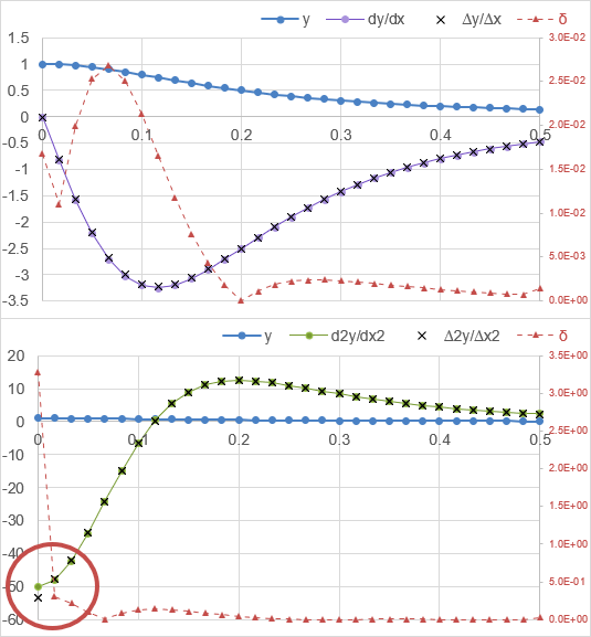
Test: Copy and Paste this LET function into a cell
=LET(
    x, L_LINSPACE(0,0.5,31),
    y, 1/(1+25*x^2),
    h, INDEX(x,2)-INDEX(x,1),
    dydx,-50*x/(1+25*x^2)^2,
    d2ydx2,5000*x^2/(1+25*x^2)^3-50/(1+25*x^2)^2,
    pdiff1,L_PDIFF(x,y,1,2),
    pdiff2,L_PDIFF(x,y,2,2),
    VSTACK(
     HSTACK("x","y","dy/dx","∆y/∆x","δ1","d2y/dx2","∆2y/∆x2","δ2"),
     HSTACK(x,y,dydx,pdiff1,ABS(pdiff1-dydx),d2ydx2,pdiff2,ABS(pdiff2-d2ydx2))
    )
)
Let δ be the error in the finite difference approximation calculated as δ1=|dydx-Δy/Δx| and δ2=|d2y/dx2-Δ2y/Δx2|. This is shown in the graph below as the dotted red line with triangle markers. From the graph we can see that the largest errors in the first derivative are occurring on the left between 0 and 0.15 (δ1≈0.025). The largest errors in the second derivative are occurring at x=0 (δ2≈3.3).
 What are our options for increased accuracy?
1. Increase the order of accuracy of PDIFF to 4 (2 additional points with a higher degree polynomial fit). This changes the first derivative error to δ1≈0.004 and the second derivative error to δ2≈0.2.
...
    pdiff1,L_PDIFF(x,y,1,4),
    pdiff2,L_PDIFF(x,y,2,4),
...
2. Decrease the step size. If we double the number of points, cutting the step size in half, we end up with δ1≈0.007 for the first derivative and δ2≈0.9 for the second.
...
    x, L_LINSPACE(0,0.5,61),
...
If we combine options (1) and (2), doubling the number of points and using order=4, we get δ1≈0.00014 and δ2≈0.032. The problem spot is still the far left edge.
3. Add a few extra points in the areas where we need higher accuracy. PDIFF gives us this flexibility because it doesn't require the step size to be constant. This is similar to refining a mesh in finite element analysis. Let's add some points close to x=0 using VSTACK and SORT to add a few specific points to the set created by L_LINSPACE.
...
    x, SORT(VSTACK(0.001,0.005,0.01,0.02,L_LINSPACE(0,0.5,31))),
...
We've added just 4 points and with the order=2, we get δ1≈0.027 and δ2≈0.22. If we combine options (1) and (3), adding the 4 extra points and changing order to 4, we get δ1≈0.0007 and δ2≈0.007. The results for this case are shown in the image below.
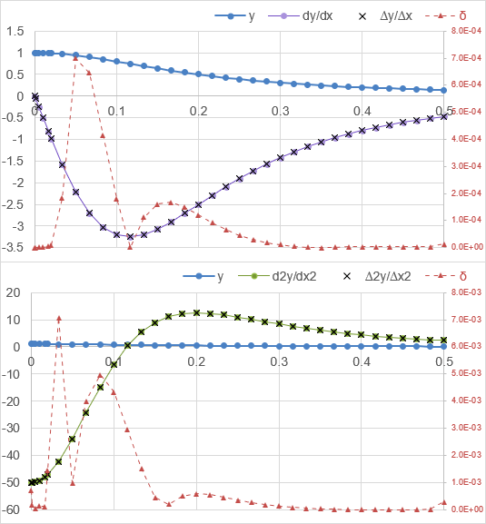
The point of this example was to demonstrate what can be achieved using fewer points, higher-order finite difference formulas, and uneven spacing.
Of course, finite difference is mainly used when you do not have the exact formulas for the derivatives. In these cases, you can do error analysis by checking how values at specific points converge as you change the step size, increase the order of the finite difference formulas, and add additional points in specific areas (mesh refinement). In general, the areas to refine are edges, inflection points, zeros, mins, maxs, etc.
Bonus: Using our known function for the second derivative, let's solve for x where the second derivative is 0 using our Newton-Raphson function.
=SOLVE_NR(LAMBDA(x,5000*x^2/(1+25*x^2)^3-50/(1+25*x^2)^2),0.12,0,0.00001)
=0.11547
=LET(
    x, L_LINSPACE(0.1,0.15,7),
    y, 1/(1+25*x^2),
    pfit, L_POLYFIT(x,y,6),
    pder2, L_POLYDER(L_POLYDER(pfit)),
    SOLVE_NR(LAMBDA(x,L_POLYVAL(pder2,x)),0.11,0,0.001)
)

Result: 0.11547
